Use py-smps to analyze size-resolved particle sensor data
py-smps is an open-source python package to help analyze and visualize data from aerosol sizing instruments such as the Scanning Mobility Particle Sizer (SMPS), Scanning Electrical Mobility Spectrometer (SEMS), and other aerosol-sizing instruments such as optical particle counters (OPCs). While it was originally developed to analyze data from research-grade instrumentation, it can also be very helpful in analyzing air quality sensor data.
In this post, we will show how py-smps can be included in your workflow, using data from a QuantAQ MODULAIR-PM as an example. Specifically, we will go over the following examples which outline common sensor workflows:
- Computing PM1, PM2.5, and PM10 values from OPC data
- Applying a custom 'counting efficiency' correction to your data
- Applying a correction factor for relative humidity
- Comparing your low-cost device to a reference instrument
1. Compute PM1, PM2.5, and PM10 values from your OPC data
The QuantAQ MODULAIR-PM sensor contains a commercially-available Alphasense OPC-N3 optical particle counter. Like other OPCs, the raw data obtained from the instrument are in units of particle number concentration (i.e., the number of particles per cubic centimeter) by bin, where each bin represents the range between two particle diameters. The Alphasense OPC-N3 has 24 size-bins ranging from 0.35 µm to 40 µm. To calculate the total integrated mass (i.e., PM2.5), you must convert the number concentration to a mass concentration and then sum the individual bins where the bin bounds are below 2.5 µm.
py-smps has this functionality integrated and computing mass loadings is simple! First, we must load the sample data and initialize an ModulairPM object:
import smps
import pandas as pd

# Load the data into a pd.DataFrame
df = pd.read_csv(
    "https://raw.githubusercontent.com/quant-aq/py-smps/master/tests/datafiles/MOD-PM-SAMPLE.csv",
    parse_dates=["timestamp"],
    index_col="timestamp"
)

# Resample to a 1min time base
df = df.resample('1min').mean()

# Initialize the ModulairPM object
obj = smps.models.ModulairPM(data=df)
Once the object is initialized, it is incredibly quick and easy to compute mass loadings between any two diameters. Below, we will compute PM1, PM2.5, and PM10 mass loadings:
# Compute PM1 assuming rho=1.65 g/cm3
pm1 = obj.integrate(weight='mass', dmin=0., dmax=1., rho=1.65)

# Compute PM2.5 assuming rho=1.65 g/cm3
pm25 = obj.integrate(weight='mass', dmin=0., dmax=2.5, rho=1.65)

# Compute PM10 assuming rho=1.65 g/cm3
pm10 = obj.integrate(weight='mass', dmin=0., dmax=10., rho=1.65)
If, for some reason you wanted to get crazy and compute PMx (PM10 - PM2.5), you could simply subtract the above computed pm25 from pm10, or you could compute from scratch:
pmx = obj.integrate(weight='mass', dmin=2.5, dmax=10., rho=1.65)One of the perks of using py-smps to do this, is that the code remains unchanged even if you are analyzing a reference instrument like a Grimm 11D or SMPS. The bin definitions will change, but all of the computations remain the same.
2. Apply a custom 'counting efficiency' correction to your data
It is completely within the realm of possibility that whatever low-cost particle sensor you may be using does not count particles with 100% efficiency relative to a reference instrument. Therefore, it may be useful to experimentally determine the counting efficiency on a size-resolved (or bin-resolved) basis and then correct your data.
Let's start with the data we imported in the above section and take a quick look at the first few rows and bins of data (number concentration):
obj.dn.iloc[0:3, 0:3]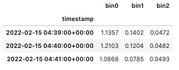
Let's say we experimentally determined that the counting efficiency was 50% for all 24 size bins of the Alphasense OPC-N3. We can use the bin_weights argument when we initialize the ModulairPM object to account for this fact:
import numpy as np

# Create an array of 1's
bin_weights = np.ones(24)

# Change all bin weights to be 2 to account for
# 50% counting efficiency
bin_weights = bin_weights * 2.

# Initialize a new object using these bin weights
newobj = smps.models.ModulairPM(data=df, bin_weights=bin_weights)

newobj.dn.iloc[0:3, 0:3]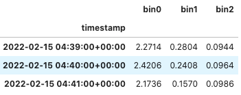
We see that the number concentration in each bin and at each point in time is exactly double what it was before! Now, when we go to compute the integrated mass values, they will also double. This is a simple example that doesn't necessarily need to be this complicated. If we know the counting efficiency is constant across all size bins, then we can just multiply the mass, right? What if it's not constant across all size bins? The bin_weights array we created above is easy to modify - you can either modify each bin individually, or create a function to compute the counting efficiency based on particle size, if that's what you wanted to do. Let's change the first few bins (those below 1 µm) and leave the rest the same:
bin_weights = np.ones(24)

bin_weights[0] = 10.	# 10% ce
bin_weights[1] = 5.		# 20% ce
bin_weights[2] = 2.		# 50% ce
bin_weights[3] = 1.2	# 83% ce

newobj = smps.models.ModulairPM(data=df, bin_weights=bin_weights)
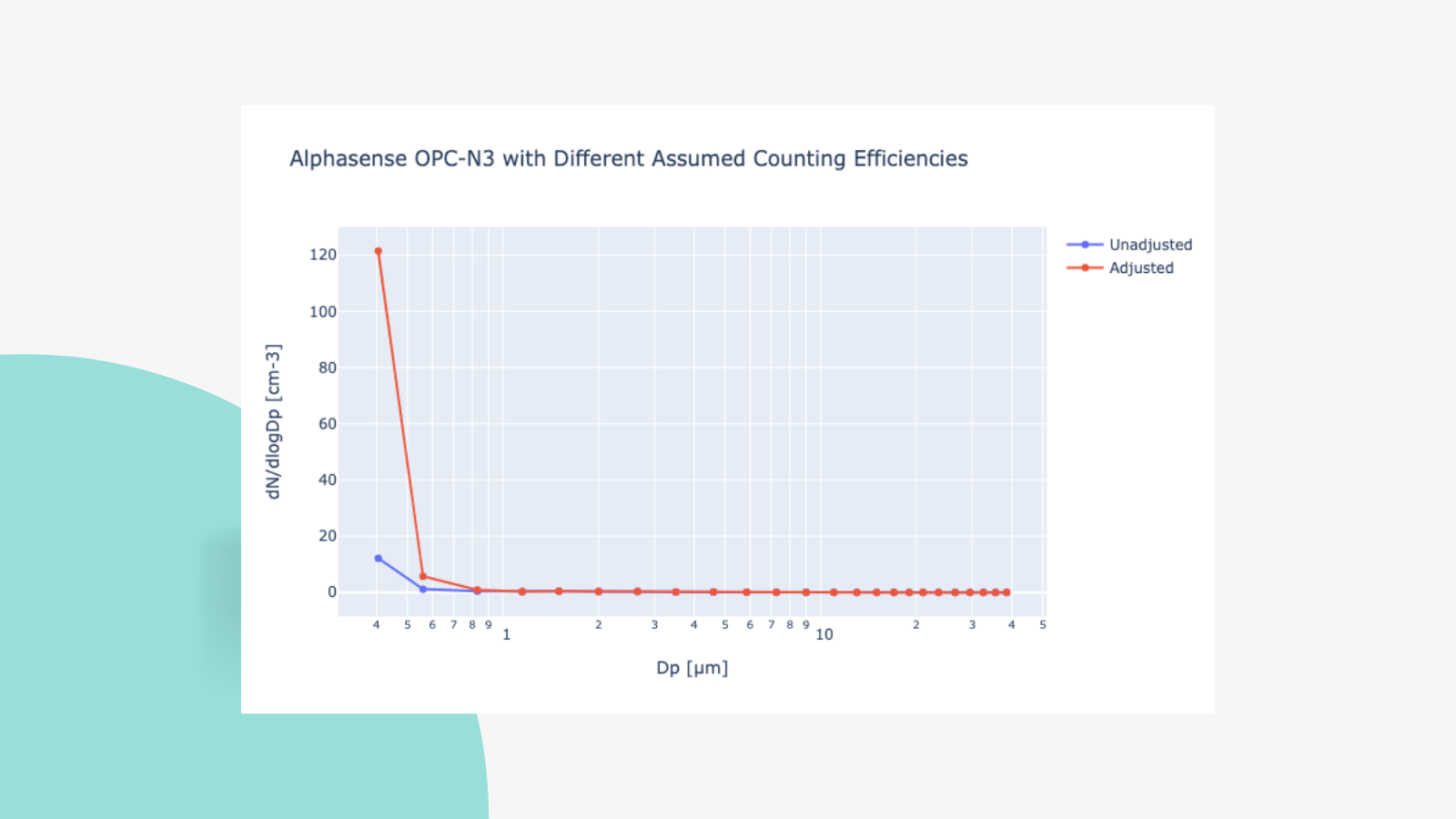
Now, if we plot the particle size distribution, we get the following:
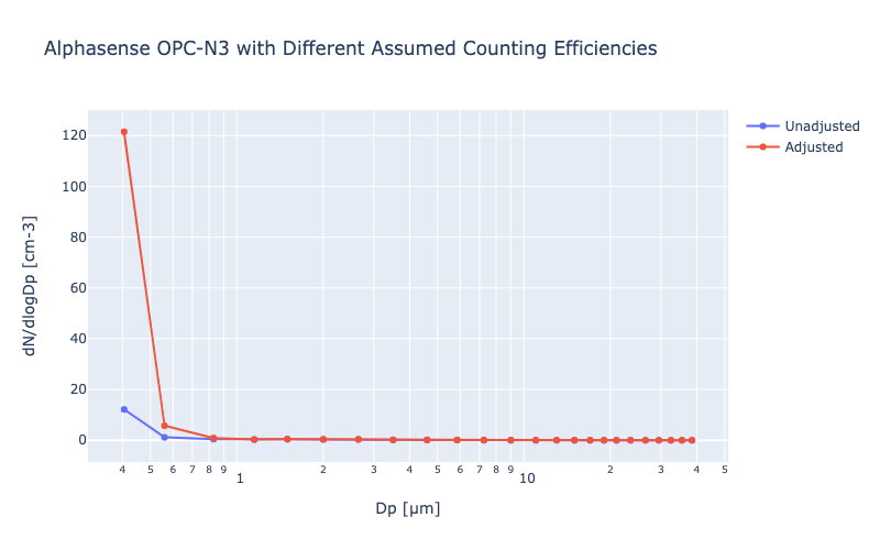
Now, when you integrate the mass (i.e., compute PM2.5), you see a ~2x increase.
3. Correct your data for hygroscopic growth
If your goal is to compute PM values and compare them to reference instruments such as a BAM or TEOM, you will want to (at a minimum) correct your underlying data for hygroscopic growth as most/all low-cost OPCs do not include in-line driers. Hygroscopic particles will take up water as the relative humidity increases and this will change the optical properties of the aerosol (i.e., refractive index) as well as their physical size. For more details on the science, check out this paper.
There are at least two papers that propose correction factors for hygroscopic growth: (1) Leigh Crilley, et al (2018) and (2) Andrea Di Antonio, et al (2018). Here, we will show how to apply the first of these corrections.
Crilley, et al (2018) Correction
The Crilley, et al correction adjusts the mass estimate at a given size cut (i.e., PM1, PM2.5, PM10) by applying an equation based on κ-Köhler theory which uses an assumed hygroscopicity parameter (κ) and the relative humidity at that point in time to compute a 'dry' mass. The equation (Eq. 5 in the paper) can be written in Python as follows:
def crilley_correction_factor(mass, kappa, rh, **kwargs):
	"""Compute the humidity-corrected mass according to
    Crilley et al (2018).

    Params
    ------
    mass: float
        Uncorrected mass value.
    kappa: float
        Kappa
    rh: float
        Relative humidity as a percent.
    rho_w: float [optional]
        Density of water.
    rho_p: float [optional]
        Density of the dry particle.

    Examples
    --------
    >>> crilley_correction_factor(100., 0.3, 85.)

    """
    rho_w = kwargs.pop("rho_w", 1.)
    rho_p = kwargs.pop("rho_p", 1.65)

    return mass / (1 + ((rho_w/rho_p)*kappa) / (-1 + (1./(rh / 100.))))
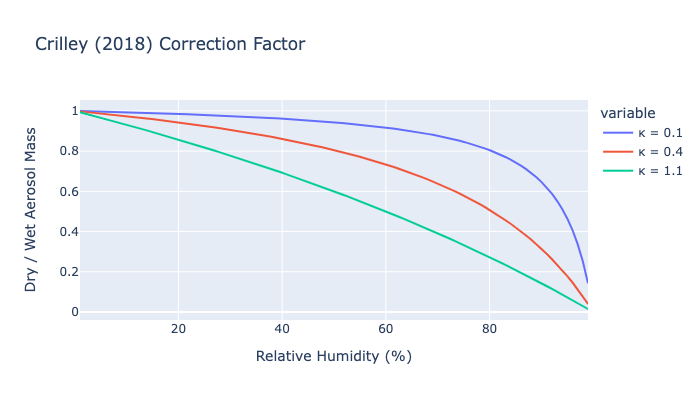
Below, we plot the ratio of dry to wet aerosol mass as a function of relative humidity for a few different κ values - we see that even at modest humidity values (~50%), the dry weight of the aerosol is just 60-94% of the initial wet weight depending on the κ value. The κ values chosen represent wildfire aerosol (κ = 0.1), urban aerosol (κ = 0.4), and marine aerosol (κ = 1.1).
Now that we have the function written, we can go ahead and apply it to our data.
import smps
import pandas as pd

# Read in the sample MODULAIR-PM dataset as a csv
df = pd.read_csv(
    "https://raw.githubusercontent.com/quant-aq/py-smps/master/tests/datafiles/MOD-PM-SAMPLE.csv",
    parse_dates=["timestamp"],
    index_col="timestamp"
)

# Define your assumed kappa value
k = 0.4

# Compute a new column called "pm25_corr"
df["pm25_corr"] = df.apply(lambda x:
	crilley_correction_factor(x["pm25"], k, x["sample_rh"]), axis=1)
While this sample dataset may not be the best example for showcasing this (the humidity is relatively muted), you now have an RH-corrected PM2.5 value using this peer-reviewed method!
4. Compare your low-cost sensor data to a reference instrument
In this context, comparing your size-resolved low-cost sensor data to a reference instrument likely means comparing the counting efficiency on a bin-by-bin basis. In this case, you will likely have a low-cost particle counter with wide bins (ex. Alphasense OPC-N3) and a reference instrument such as a Grimm 11D or an SMPS with much more size-resolving power. To compare the two instruments, it is helpful to put them on the same size-base (i.e., make their bins overlap perfectly). Using the integrate function in py-smps, this is simple.
To do so, we will need both datasets as their respective objects:
import smps
import pandas as pd

# Read in the sample MODULAIR-PM dataset as a csv
df = pd.read_csv("<filepath here>")

# Create the MOD-PM object
opc = smps.models.ModulairPM(data=df)

# Read in your reference data here
df = pd.read_csv("<filepath here>")

# Read in the SMPS dataset
ref = smps.io.Grimm11D(data=df)
Next, we will iterate over the bins of the low-cost OPC, since they are larger, and compute the integrated number concentration from the Grimm 11D across the same size range:
for i, (lb, _, rb) in enumerate(opc.bins):
	# compute the number conc. between the left and right boundaries
    pnc = ref.integrate(weight='number', dmin=lb, dmax=rb)

    # compute the mean counting efficiency in the bin
    ce = (opc.dn["bin{}".format(i)] / pnc).mean()

    # print out the results
    print ("OPC bin{} = %.3e".format(i, ce))
It's as easy as that! For more tips on data science pertaining to air quality sensors, make sure to follow the QuantAQ blog.

